Technical Article

An Overview of Integral Gain

July 24, 2020 by David Peterson

This article discusses the meaning of integral gain and how to calculate integral gain to achieve better control results.

Some control systems can rely on the simple mathematics of a proportional system to achieve the desired results. However, no amount of proportional gain can yield perfection with an instant response - in fact, no real-world system can do so. But if a better amount of control is to be achieved, integral gain is often called on to bring better results.

The Meaning of Integral Gain

Most control systems use some sort of feedback to provide variable output signals to a process. These outputs are carefully calculated using a variety of terms coupled together in order to provide output voltages to hydraulic valves, heaters, motor controllers, and any other device that needs something more precise than a simple on/off control.

Calculating this output signal is the combined effort of several mathematical terms relying on the amount of error in the system. As described in many texts, the error is the difference between the intended system target value (SetPoint SP) and the current sensed value from the process (Process Variable PV).

$$Error=SP-PV$$

The most basic term used in this output calculator uses a multiplying constant called Proportional Gain, which is a direct ratio of error to the output signal. A small error indicates approaching the target, so the output signal begins to level off. Otherwise, the system would drive at full throttle until shooting past the target and requiring a return. This concept is appropriately called ‘Overshoot.’

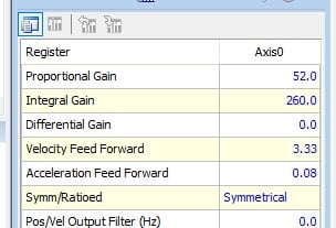
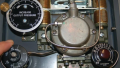
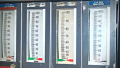
An example of a tuned output display with parameters including Integral Gain. Many times, the software is tuned by a built-in algorithm, while other times, it is necessary to manually calculate gain values.

There are two key weaknesses seen in Proportional control systems which use an increased Proportional Gain (Kp) to provide stabilization. First, the output is slower to reach a final settled value and that final settled value may not reach the target, providing Steady-State Error.

A method of solving this problem is by adding a second common term of Integral Gain (Ki) which can counter those effects to some extent but does provide weaknesses of its own which must be balanced beside the Kp effects.

Calculating Integral Gain

The process of integration is a calculus concept, but the reality is that it doesn’t require a math background to understand the method used. Technically, integration is a continuous addition of the area underneath or between curves defined by equations. The difference is that with a real-world system, the whole purpose is to compensate for external changes that influence operation.

If the system was completely predictable and calculatable in 100% of cases, there would be no reason for feedback and a continuous slight change of the control output. In reality, the error difference between SP and PV changes every time the system runs, so calculations based on smooth, equation-driven curves do not work.

Even though it may not fit a predictable mathematical curve, the Integral term still uses this ongoing addition or ‘summation’ of error. It may be displayed as shown below:

$$Integral~Term=K_i \times \Sigma Errors$$

Although this is the correct notation, it doesn’t mean much to a real system. In reality, the process would look more like this, with each error reading taken in rapid succession with each other:

$$Integral~Term=K_i \times (error1+error2...+errorN)$$

As you can see, the larger the error over time, the larger the contribution from the integral term. The $K_i$ is simply a multiplier number with units based on the dimension of the target process variable and time, a multiplier which might range from small decimal values to larger values depending on the size of the system. The error might be on the magnitude of fractions of mm for the motion of a hard drive needle, or it might be a large number of inches for the location of a hydraulic cylinder, so there is no single value of gain which can be applied to every system.

Effects of Integral Gain

Accumulation of error takes time to happen, so the result of Integral Gain ($K_i$ ) is not seen right away when the system SP is entered. At that moment, the error begins to build.

A large value of $K_i$ will cause a system to reach the set point faster once there has been a slight buildup of error. This is especially useful if the system has begun to level off before reaching the set point because of a large proportional gain factor. In this case, the error will start climbing, but at a consistent rate.

A problem with a high value of $K_i$ is a re-introduction of overshoot as the system responds to error, even if close to the SP.

Visually, the effect of a system with only $K_i$ would appear at the beginning as an uncompensated system (just like it would with no gain at all). The rate of change would be fairly linear for a short time. Very quickly, as error builds, the rate of change of the system would increase, accelerating toward the SP. Overshoot would most certainly appear before the system settles.

One main benefit is that even with the oscillations, the system will finally settle right on the target SP, since even a little bit of steady-state error will eventually cause a rise in output, enough to get to the SP.

In one special case of accumulating output, if the system cannot physically reach the SP, like a temperature-controlled system that is cooling too fast to ever reach the target SP, then the error would keep climbing. The system would keep trying to drive the heating element higher and higher beyond its physical limits, for example, sending 15 volts to control that only accepts up to 10 volts.

When it comes time to cool down, the heater control output will be reduced, but it will take some time before the voltage control falls to 10 volts, and finally, after that, the system will actually respond. This is called ‘Integral Windup’ or ‘Reset Windup’ and must be compensated out of the equation if this condition is met.

Because of the fast rise in output, it is rare to ever see an Integral system by itself. They will always be paired either with a Proportional term (PI system) or with a third additional Derivative term (PID system).

Interested in learning more about PID controls and gain?

Articles:

Textbook: