Facebook
 Google
 GitHub
 Linkedin
The Difference Between Linear and Nonlinear Finite Element Analysis (FEA)
Finite element analysis (FEA) helps foster our understanding of the physical phenomena within engineering designs. Dive into FEA’s foundation and how it handles linear and nonlinear applications.
What is Finite Element Analysis (FEA)?
Finite element analysis (FEA) is a simulation process used by engineers to divide complex boundary value problems (BVP) into manageable, predictable pieces, where the relationship between stress and strain or force and displacement can be described. A BVP is a mathematical problem where the initial boundary conditions are known and are used to solve points throughout the region. Common BVPs include structural analysis, heat and fluid flow, and electrical potential, all of which can be analyzed in static and dynamic conditions.
The pieces that FEA creates are called elements, and the total number of elements forms a mesh. The user can manually or algorithmically alter the mesh density based on the complexity of the model by increasing mesh density on joints, curves, or important areas within the model. Generally, it is good practice to begin with a coarse mesh density to give a rough understanding of the key points in the model where further mesh refinement can be done.
Depending on the model’s size, there could be hundreds, thousands, or millions of elements, increasing the simulation time from a couple of minutes to multiple days, depending on the computing power available. A proper understanding of meshing and mesh refinement can save hundreds of hours of computing time.
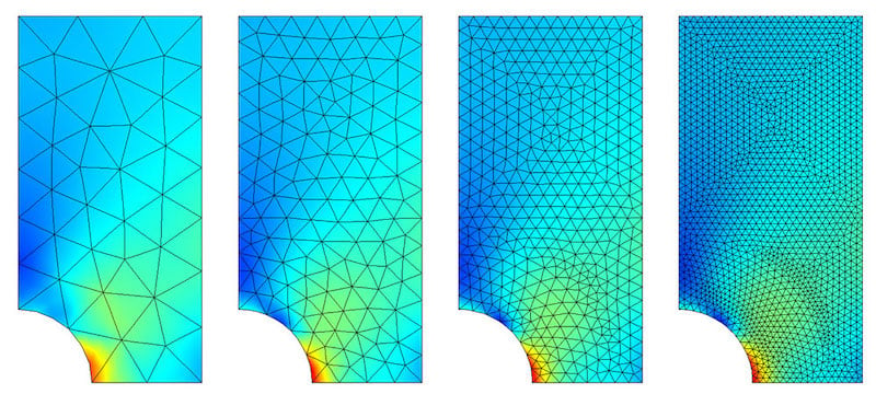
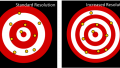
Figure 1. Visualization of increasing mesh density on a steel plate. Image used courtesy of Comsol
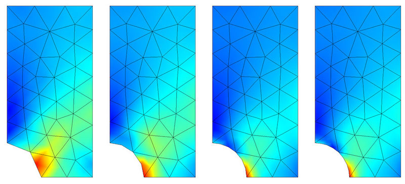
Figure 2. Visualization of local adaptive meshing. Concentrating the mesh density around the area of highest stresses. Image used courtesy of Comsol
After each small piece is mathematically described, they are re-assembled and linked together. The relationships between elements are analyzed through a series of compatibility and/or continuity equations, forming a larger system of equations that populate a matrix. For example, knowing the forces applied to a structure and the stiffness of the structure, FEA can calculate the displacements of each element by solving the system of equations within the matrix. Stresses and strains can be solved in a similar fashion.
Linear Finite Element Analysis
Linear FEA makes several key assumptions that simplify the overall analysis.
- First, the model only undergoes small deformations and deflections based on the applied forces.
- Second, the material does not experience any plastic deformation or creep due to loading.
- Third, the boundary conditions remain the same and do not change throughout the simulation.
Small deformations mean that the material resides within the linear portion of the stress-strain curve (following the material's elastic modulus). This means that the material remains in its elastic state, does not experience any plastic deformation, and deflection can be calculated using Hooke’s Law.
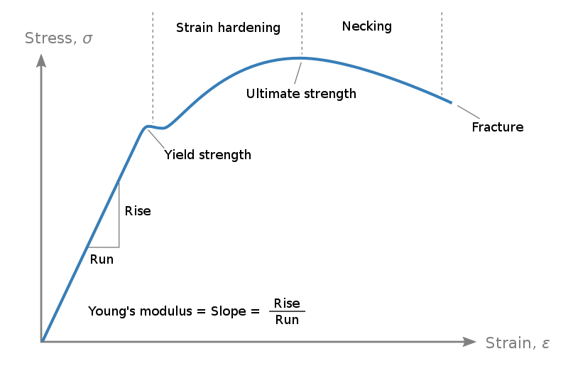
Figure 3. Stress vs. strain curve, highlighting the linear behavior of a material until reaching the yield strength point; once beyond, the material begins to behave nonlinearly. Image used courtesy of Nicoguaro
When visualized in a curve, the software, unless otherwise specified, assumes the material continues linearly without yielding or plastically deforming, which can result in massive simulation errors. As an object or model moves throughout a simulation, the boundary conditions can change. For example, a cantilever beam close to the ground might bend until it touches the ground, resulting in a new set of boundary conditions.
Additionally, the simulation will often struggle to simulate time-dependent factors, such as forces that increase over time or sporadic changes in temperature. Simply put, linear FEA will be accurate for simple scenarios, with small, static deformations in the model that remain consistent throughout the simulation.
While extremely useful, FEA can fall into the trap of "garbage in, garbage out." This means that a poorly prepared and setup simulation (through boundary conditions, material specifications, or improper consideration of linear and nonlinear effects), the data collected from that simulation will most likely be erroneous, leading to misunderstandings and a large waste of time and money. So, any FEA user must spend the time to consider all the effects on the model, both linear and nonlinear.
Nonlinear Finite Element Analysis
Nonlinear FEA often provides a more realistic approach to simulations. Specific projects may allow for linear analysis, but in most cases, nonlinear techniques provide more accurate data. As mentioned above, nonlinear problems can be classified into three major categories.
- Geometric nonlinearity, where large deflections create nonlinear behavior in the model
- Material nonlinearity, such as the plasticity of the model or creep within the material
- Nonlinear boundary scenarios, where the initial boundary conditions change based on the movement of the model
When these cases are present, the software uses a nested iterative process to solve the changing system of equations created by the elements within the model. This is unlike linear FEA, where the system of equations does not change during the solution process. Once the model deforms, has new boundary conditions, or reaches strains beyond the linear range of the force-displacement curve, the software must solve a new set of equations. Various mathematical methods are derived to perform iterations and optimizations of FEA, including the Newton-Raphson method and the Broyden-Fletcher-Goldfarb-Shanno method.
There are special considerations where current nonlinear methods continue to struggle. For example, buckling offers a very difficult scenario for most nonlinear methods to compute. Buckling is defined as the sudden, spontaneous deformation of a material under a load. It is difficult to predict and model, but adding methods such as the arc-length method continues to produce more accurate results.
FEA, when properly implemented, is a powerful and efficient tool that can provide realistic data about how a design will work prior to a costly construction process. However, a user must accurately consider both linear and nonlinear aspects of the project.
Related Content